Note · 2026-09-17

Point it at a warehouse, get an analyst trained on the answer

Every company asks why a number fell, and no company records the answer. That is the whole problem with training an agent to investigate: your warehouse knows what happened, never why. Last Tuesday’s drop has no label, and without a label there is no reward.

This note describes what we built to get round that, and walks through one execution of it end to end, with the numbers from that run rather than from a description of it.

The problem

“Revenue fell 14% last week — why?” is one of the most common questions in any business and one of the hardest to answer well. An analyst decides where to look first, reads what comes back, forms competing explanations, tests them, drops the wrong ones, and stops when the evidence is enough. There is no single correct path, and a wrong first move wastes the whole investigation.

A capable model with database access can already do this passably. The question we care about is whether it can learn to do it better from its own outcomes — and that runs into the wall above. The usual workarounds make it worse rather than better. An LLM judge scores confident writing rather than correct answers. Human labels cost more than the analysis they replace. Historical incidents are few, inconsistent, and written up after the fact by whoever was wrong first.

The approach

We generate a twin of the warehouse: the same table and column names, the same dimension vocabularies, roughly the same scale, and entirely synthetic rows. Into that twin we inject causes. Because the world is generated deterministically, it can be rebuilt with one cause removed and everything else identical — and the change in the metric is that cause’s exact contribution. That is the reward, and it is arithmetic rather than opinion.

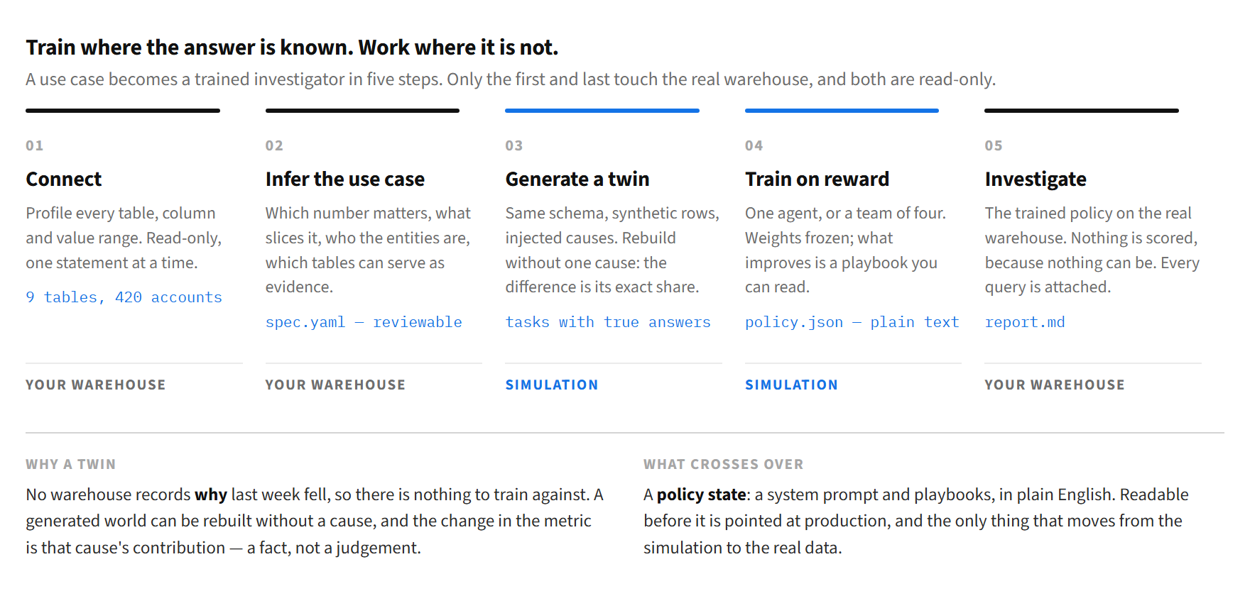
Figure 1. Only the first and last steps touch real data, and both are read-only. Training happens entirely in the simulation.

What crosses from the simulation to the real data is not a model — the weights never change — but a policy state: a system prompt and playbooks of learned lessons, in plain English, which a person can read before it is pointed at production.

Step 1 and 2: connect, and work out the use case

Two things are supplied by a person: a connection string, and which number matters.

llm-rle studio init duckdb:///warehouse.duckdb --list-kpis
llm-rle studio init duckdb:///warehouse.duckdb --kpi 0 \
    --kpi-name "weekly paid invoice revenue" --out specs/revenue.yaml

Profiling reads every table, column, value range and vocabulary — never rows. Inference then works out the fact table, the metric and its date column, the dimensions worth slicing by, the entity table behind the fact rows, and which tables can serve as evidence for which kinds of failure.

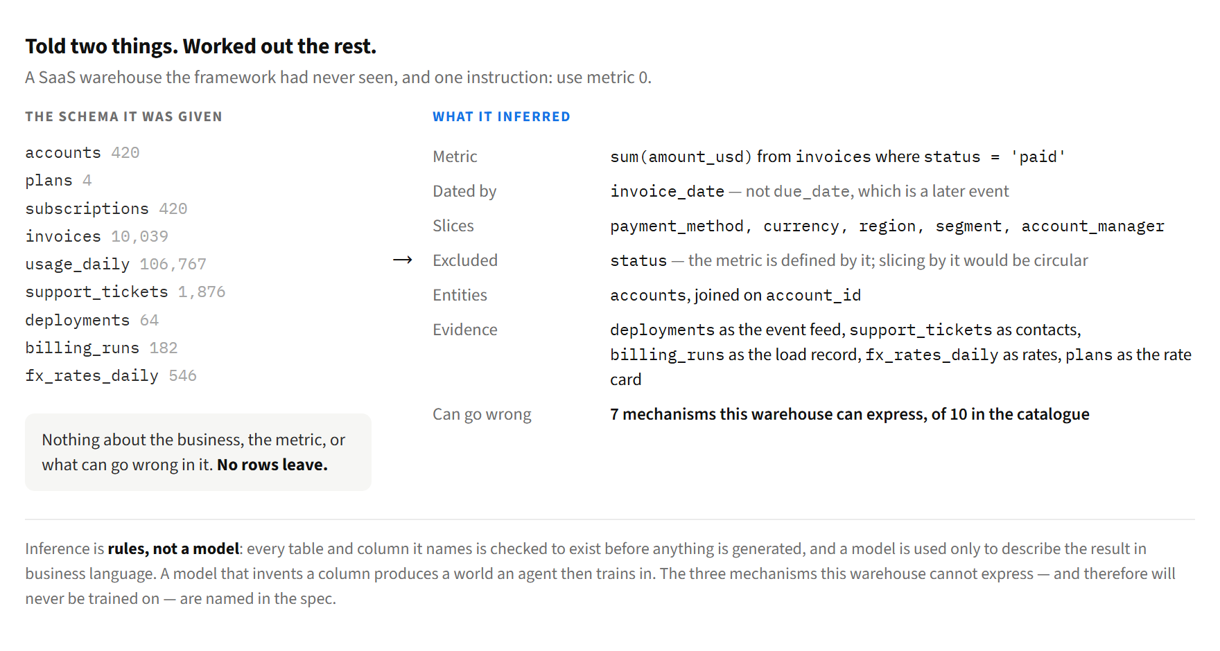
Left: the nine tables of a SaaS warehouse with row counts. Right: what the studio inferred - the metric is the sum of paid invoice amounts dated by invoice_date rather than due_date; five dimensions; status excluded because the metric is defined by it; accounts as the entity table; five evidence roles; seven of ten catalogue mechanisms available. — Figure 2. Run against a SaaS warehouse written independently of the framework, in a different domain from anything it had seen. All seven role assignments correct, from the schema alone.

Two decisions carry most of the weight here. Inference is rules, not a model: a model that invents a plausible column name produces a world an agent then trains in, so a model is used only to write business-language descriptions, and every table and column named is checked against the schema before anything is generated. And the result is a spec file that a person reviews — which metric, which slices, and what the generator believes can go wrong in this business.

Failure mechanisms are gated on what the schema can express. A warehouse with no currency column never gets currency-translation faults; one with no load-audit table never gets pipeline gaps. In this run, seven of the ten mechanisms in the catalogue were available and the other three are named in the spec as out of scope, so the spec is honest about what it does not cover.

Step 3: generate a world that can be rerun

A week down 13.9 per cent, a gap of 9,143. Rebuilding the week without the aborted billing load recovers 3,451, which is 38 per cent of the gap; without the enterprise churn, 2,756, which is 30 per cent; without the misconfigured promotion, 2,083, which is 23 per cent. Two decoys recover exactly zero. — Figure 3. Each cause's share, measured by rebuilding the same week without it. The decoys measuring exactly zero is the check that the simulation is sound.

Tasks are generated across the splits that separate a lucky agent from a capable one: familiar cause types, two causes at once, cause types deliberately held out of training, and cases with a decoy planted to mislead. Each generated investigation reads like the real thing, and carries an answer the agent never sees:

test_recovery-0 — weekly paid invoice revenue for 2026-09-07 to 2026-09-13 was $270,427, 28.8% below the average of the previous 4 periods ($379,813). Investigate the data, identify the root causes of the decline, estimate each cause’s share, and submit your conclusion.
Truth, never shown: a processing failure scoped to currency=AUD worth 1.20 of the decline, plus two decoys worth exactly nothing.

Generation tunes itself to the warehouse, because the same “85% of this slice fails” is a rounding error in one business and an outage in another. Magnitudes are tuned until the metric falls believably, a cause whose slice is too small to matter is widened, and a week whose own variation would credit a cause with more than the whole decline is re-rolled. Fourteen tasks for this use case took 23 seconds and no model calls.

Step 4: train, and read what was learned

llm-rle studio train specs/revenue.yaml --policy single
llm-rle studio train specs/revenue.yaml --policy swarm

Both arms train with the model’s weights frozen. What improves is a playbook, learned by contrasting a high-reward investigation against a low-reward one on the same case and writing down what separated them. The single agent learned eight lessons; the first, verbatim:

Start with broad decomposition: run describe_schema, then kpi_breakdown on a few high-yield dimensions (segment, region, payment_method, currency) and identify the single slice contributing most of the KPI decline.

The swarm is a lead plus three specialists whose briefs are written from this warehouse’s own tables — one owns breakdowns, one owns the accounts behind the metric, one owns whether the value was lost or merely not recorded. Each keeps its own playbook plus a shared one. Its measurement specialist learned:

For a KPI defined on paid invoices, start with one compact invoices check comparing current vs baseline by status, count(*), and sum(amount_usd).

On eight unseen tasks in the twin, the single agent scored 0.50 reward and 38% fully correct; the swarm 0.29 and 12%, at nearly double the tokens. With six training tasks and one seed that is a direction rather than a verdict — but it does show the generated environment discriminates instead of scoring everything alike.

Step 5: investigate the real warehouse

llm-rle studio investigate specs/revenue.yaml --db duckdb:///warehouse.duckdb \
    --policy single --policy-state runs/…/policy/final.json --out report.md

The agent is told what the metric actually did in the most recent complete period and investigates with the same tools it trained with. There is no ground truth here and the framework does not pretend otherwise: nothing is scored. The output is a conclusion — each cause with a scope, a share and its evidence — followed by every query it ran, in order, for a person to check. From the generated report, after 28 queries and 48 seconds:

The 7.0% KPI decline was driven almost entirely by a processing problem in EMEA card payments. After the 2026-09-06 billing deployment that migrated EU card processing to a new provider, the count of paid EMEA card invoices fell sharply, while invoice values did not — pointing to transactions failing to complete rather than weaker demand or lower pricing.

That conclusion is correct. The demo warehouse was built with exactly that fault, and with a small-account churn in the same week as a decoy, which the agent examined and rejected. It was told neither.

One execution, end to end

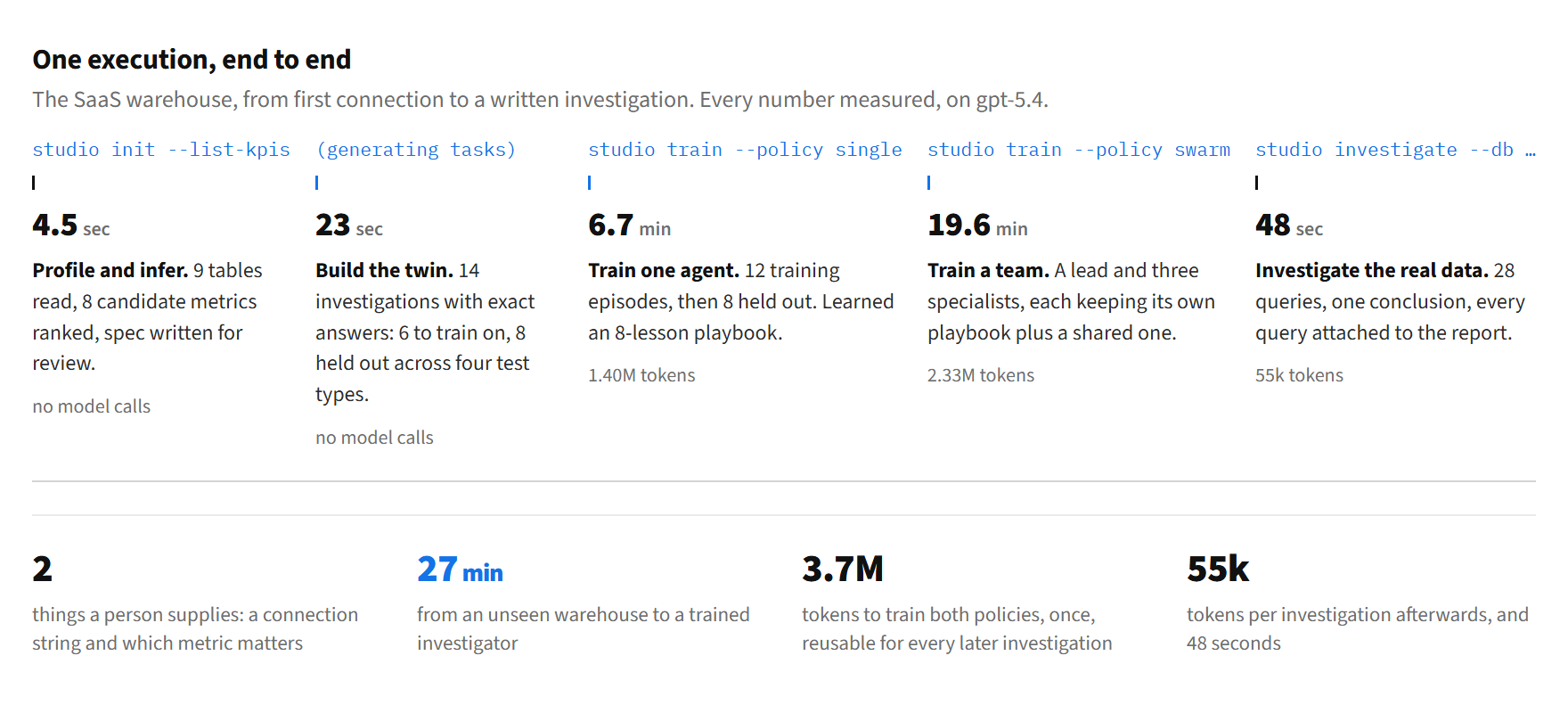
Figure 4. Every number measured on the run. Training is paid once; investigations afterwards cost 55k tokens each.

Twenty-seven minutes from an unseen database to a trained investigator, of which four and a half seconds were spent reading the schema and twenty-three generating the training world. Both of those steps make no model calls at all.

The case that separates them

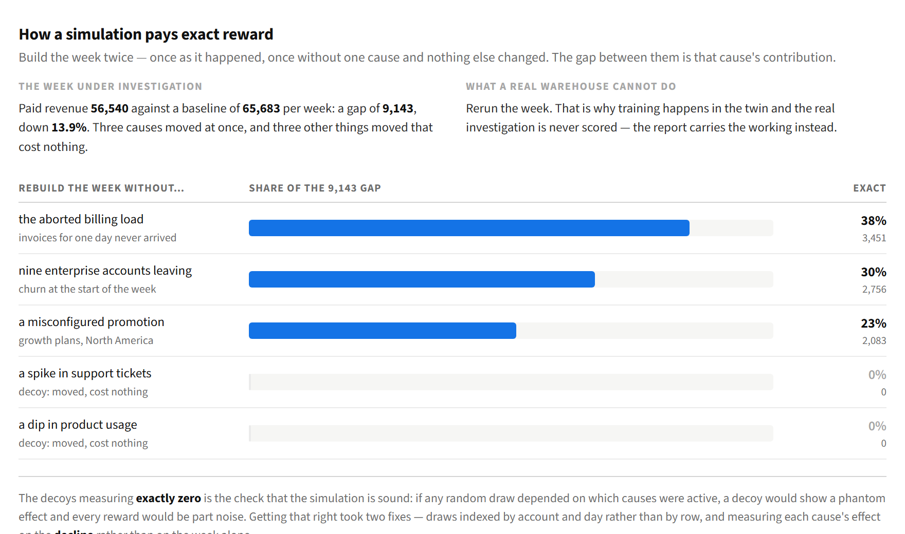
A single-cause week turned out to be a poor test: all three arms found it, and it separated nothing. So the demo warehouse also carries a week with three simultaneous causes from three different families — an aborted billing load, enterprise accounts churning, a misconfigured promotion — alongside three decoys that move and cost nothing. Because it is simulated end to end, each share is exact and the arms can be scored on data that looks real.

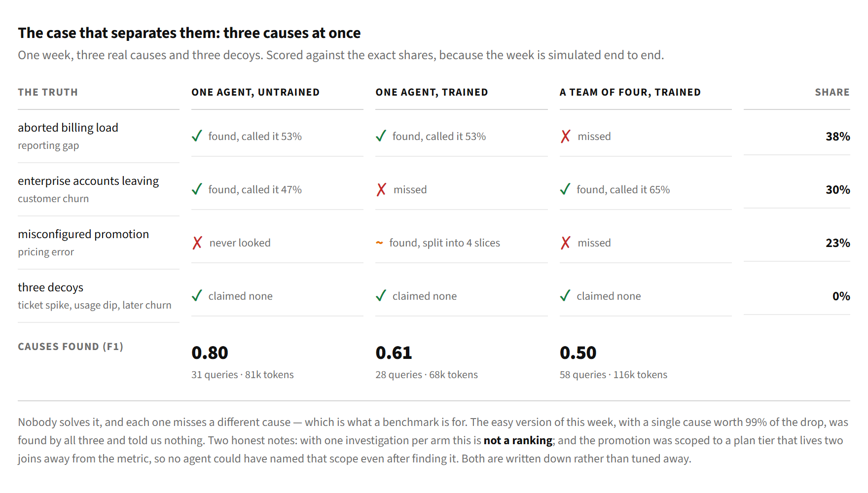
Scoreboard for the three-cause week. The untrained agent found the billing load and the churn but never looked for a pricing change, scoring 0.80. The trained agent found the billing load and the promotion, split into four slices, but missed the churn, scoring 0.61. The trained team found only the churn, scoring 0.50. All three correctly claimed none of the three decoys. — Figure 5. Each arm misses a different cause, and none of them solves it — which is what a benchmark is for.

Two honest notes travel with that table. With one investigation per arm it is not a ranking. And the promotion was scoped to a plan tier that lives two joins from the metric, so inference never made it a dimension and no agent could have named that scope even after finding it — a real limitation of the current system, written down rather than tuned away.

What is enforced, and what it cannot do

Four properties are enforced rather than intended. The connection reads only: every statement is checked before it runs — one statement, SELECT or WITH only, no DDL or DML — and is opened read-only where the driver allows. There is no tool that writes: the agent can query and submit a conclusion, and nothing else. Your data stays put: the spec carries schema, dimension vocabularies and summary statistics, never rows, and never free text — notes, titles and descriptions stay in the warehouse. Credentials never enter a spec or a report.

What it cannot do yet, in the order the limitations bite: the twin generates a star schema, so event-sourced or heavily normalised warehouses are simulated more loosely; dimension inference walks one join, so a slice defined two hops away cannot be named; one metric per spec; and training quality is bounded by whether the catalogue’s mechanisms resemble how the business actually fails, which is the judgement the spec review exists for.

One more thing worth saying plainly. The first training run in a generated twin scored 0.016 mean reward with zero successes, while the same untrained agent investigated the real warehouse correctly. Every reason was in the generator or the grader, not the agent: all-or-nothing scoring of near-miss labels; a noise floor of 5% against a 4% minimum decline, so a “task” could be pure variation; a world that grew into the question; and magnitudes fixed in the catalogue rather than tuned per warehouse. Two more were caught before that — a per-process random seed that made cached tasks describe data that no longer existed, and the twin copying the real warehouse’s note text into the spec. A generated environment is a piece of software like any other, and it is wrong until it is checked.

Where this goes

Three things next, in order. Breadth: a second and third warehouse in unrelated domains, to test the inference rather than the twin — the generator is the easy half, recognising an unfamiliar schema is the hard one. Depth: more training budget on one use case, several seeds of the three-cause shape as held-out tasks, and a cost-matched swarm arm, enough to turn “0.80 against 0.61” into a result rather than an anecdote. Reach: two-hop dimensions, more mechanisms in the catalogue, and a scheduled mode that investigates the weekly number and writes the report before anyone asks.

This generalises the hand-built arena behind two earlier notes — the pilot and the swarm comparison — from one environment somebody wrote by hand to one the framework writes for whatever warehouse it is pointed at. If you work on investigation or root-cause analysis over a data warehouse, we would like to hear from you.

All notes